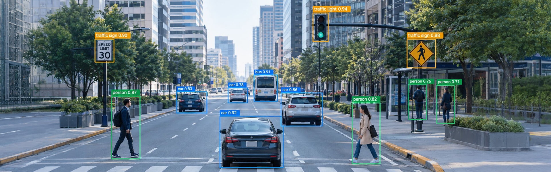
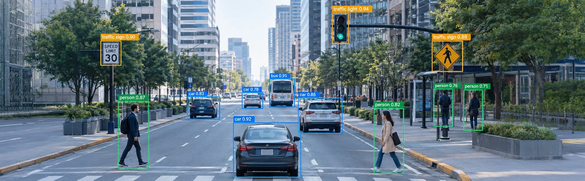
Object detection finds what is in an image and where it is. This guide explains backbones, region proposals, NMS, and mAP in plain terms, then covers the part most guides skip: how bounding box annotation rules, class taxonomy, and label quality decide what the model can actually learn.
Contents
- Key Takeaways
- What Object Detection Does
- Detection vs Classification vs Segmentation
- How Object Detection Works, Stage by Stage
- The Three Families of Detection Architecture
- What the Model Actually Learns From
- Annotation Decisions That Change Your mAP
- How Detection Accuracy Is Measured
- Why Detectors Fail in Production
- How Much Labeled Data You Need
- Do Foundation Models Remove the Need for Labeling?
- Where Object Detection Is Used
- Conclusion
- Frequently Asked Questions
Object detection is a computer vision task that finds every instance of a target object in an image or video frame and returns its position. For each detection, a model outputs four bounding box coordinates, a class label, and a confidence score between 0 and 1.
A classifier can tell you a photo contains a forklift. A detector tells you there are three forklifts, where each one is, and how sure it is about each. That difference is why detection sits underneath most production computer vision: counting, tracking, inspection, safety monitoring, and driver assistance all need coordinates, not just categories.
This guide covers how detectors work, how their accuracy is measured, and what it takes to train one on your own data. That last part gets the most space, because it is where most projects actually succeed or fail and where most explanations stop short.
Key Takeaways
- A detector returns box coordinates, a class label and a confidence score for every object it finds. Everything else is post-processing.
- Localization is learned by regression against human-drawn boxes. The model has no other source of truth about position.
- All architectures run the same five stages: feature extraction, candidate generation, classification and box regression, filtering, output.
- mAP@0.5 measures whether you found the object. mAP@0.5:0.95 measures whether your boxes are tight. A large gap between them usually points at loose or inconsistent annotation.
- Guideline decisions about occlusion, truncation, minimum object size and class taxonomy affect accuracy more than swapping one modern architecture for another.
What Object Detection Does
Object detection takes an image and returns a list. Each entry in that list has the same shape: coordinates, a class, and a confidence value.
A single prediction looks like this in practice:
class: forklift
box: x=412, y=196, width=178, height=240
confidence: 0.91
Everything downstream is built on that list. Counting is the length of the list. Tracking is matching entries across frames. Zone alerts are geometry against the coordinates.
It helps to be blunt about what the model is doing. It has no concept of a forklift. It has learned a pattern of shapes, edges, textures and spatial relationships that appeared inside boxes labeled “forklift” in its training data, and it is matching regions of a new image against that pattern. IBM’s explainer makes the same point: detectors classify aggregates of visual properties, not objects.
Two properties matter for planning. First, detection is instance-level: ten cars produce ten predictions, not one “cars” label. Second, it is closed-set by default. A detector trained on 12 classes will never return a thirteenth, no matter how obvious the object is to you.
Detection vs Classification vs Segmentation
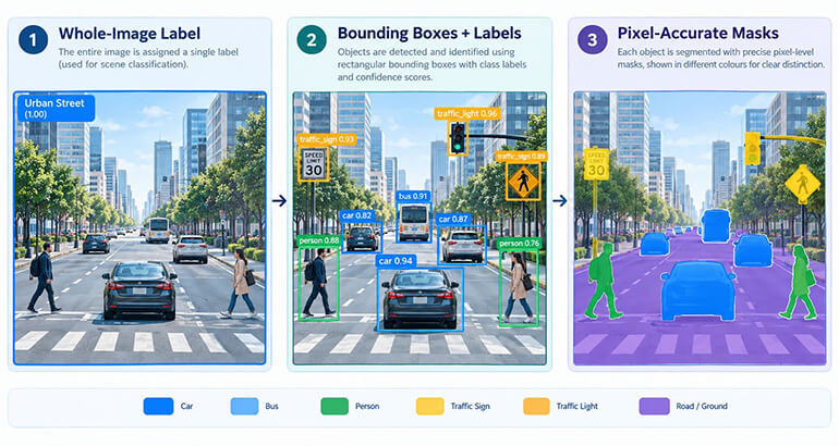
These three tasks get confused constantly, and picking the wrong one is an expensive mistake because each needs a different kind of annotation.
| Task | Question answered | Output | Annotation needed | Relative labeling cost |
|---|---|---|---|---|
| Image classification | What is in this image? | One label per image | Tag per image | Lowest |
| Object detection | What is here and where? | Box, class and confidence per instance | Bounding box per object | Low to moderate |
| Instance segmentation | What is here and what is its exact shape? | Pixel mask per instance | Polygon or mask per object | High |
| Semantic segmentation | Which class does each pixel belong to? | One class per pixel | Full-scene pixel labeling | Highest |
Pick detection when position and count are enough. Pick segmentation when shape, area or boundary precision is the point, such as measuring a defect or separating touching objects. The accuracy and cost trade-off between the two is covered in detail in this comparison of bounding box and polygon annotation.
A common mistake is specifying boxes and then discovering the product needs area measurement. Re-labeling a dataset from boxes to polygons is not an adjustment. It is a new annotation project.
How Object Detection Works, Stage by Stage
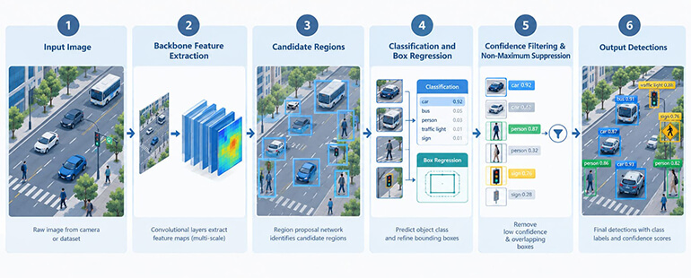
Every detector, from Faster R-CNN in 2015 to the transformer models shipping now, runs five stages. The architectures differ in how they handle stages 2 and 4.
- Feature extraction. A convolutional or transformer backbone processes the image and produces feature maps. Early layers capture edges and texture. Deeper layers capture shapes and object-level patterns. The image is down-sampled heavily along the way, which is the root cause of most small-object failures.
- Candidate generation. The model proposes places an object might be. Two-stage models use a region proposal network to score thousands of candidate regions by “objectness” and pass the best ones forward. One-stage models tile the image with anchor boxes of preset sizes and ratios, or, in anchor-free designs, predict directly from each feature map location. Transformer detectors skip both and use a fixed set of learned object queries.
- Classification and box regression. For each candidate, the model predicts a class distribution and a set of coordinate offsets. The offsets are what turn a generic candidate into a tight box around the actual object. This is the regression step, and it is trained by comparing predictions against human-drawn ground truth.
- Filtering. The raw output is far larger than the number of real objects, and most of it is duplicates and low-confidence noise. Two filters clean it up. A confidence threshold drops predictions below a cutoff, commonly 0.25 to 0.5. Non-maximum suppression then removes duplicates: it keeps the highest-scoring box for a class and deletes any other box overlapping it by more than an IoU threshold, usually 0.5 to 0.7.
- Output. What survives becomes the final detection list.
Stage 4 is worth understanding because it has a direct operational consequence. In a crowded scene with genuinely overlapping objects, such as a dense parking lot or a shelf of stacked boxes, aggressive NMS deletes real detections. Loose NMS returns duplicates. There is no setting that is right for both, which is one reason newer models have moved away from NMS entirely.
The Three Families of Detection Architecture
The old one-stage versus two-stage split no longer covers the field. Query-based transformer detectors are a third family, and since 2025 they have led the accuracy benchmarks.
| Family | Examples | How It Localizes | Typical Strength | Typical Weakness |
|---|---|---|---|---|
| Two-stage | R-CNN, Fast R-CNN, Faster R-CNN | Region proposal network, then per-region classification | Strong localization, still a solid research baseline | Slower, more complex to deploy |
| One-stage | YOLO family, SSD, RetinaNet | Dense prediction over anchors or feature map points in a single pass | Fast, small, deployable on CPU and edge devices | Historically weaker on small and overlapping objects |
| Query-based transformer | DETR, RT-DETR, RF-DETR | Fixed set of learned queries attending over the whole image | Highest accuracy, no NMS needed, strong on crowded scenes | Larger parameter counts, GPU-oriented |
Current published benchmarks give a sense of the spread. RF-DETR is the first real-time detector to exceed 60 mAP on COCO, with its largest variant reporting 60.1 COCO AP at 17.2 ms and its L variant 56.5 AP at 6.8 ms, measured on an NVIDIA T4 with TensorRT at FP16. On the efficiency side, YOLO26 reports 40.9 to 57.5 mAP on COCO at 1.7 to 11.8 ms T4 latency.
Treat those numbers as a starting point for shortlisting, not as a prediction about your data. COCO has 80 everyday classes and large, well-lit objects. A model’s COCO ranking says little about how it will handle gray scale ultrasound frames or overhead warehouse footage. For a deeper architecture-by-architecture comparison, Hitech BPO maintains a benchmark roundup of object detection models that tracks the same leader-board figures.
The practical guidance is short. If you have GPU headroom and accuracy leads, start with a transformer detector. If you are deploying to CPU or an edge device, start with a small YOLO variant. Then stop tuning the architecture and go work on the dataset, which is where the remaining accuracy is hiding.
What the Model Actually Learns From
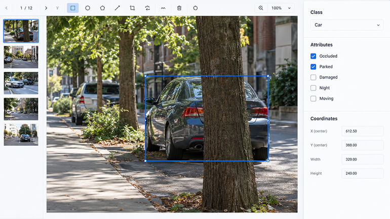
Here is the part most explanations skip. A detector has no innate sense of where objects are. It learns coordinates by being shown thousands of examples of humans drawing boxes and adjusting its weights until its predicted coordinates match theirs.
That means the annotation is not preparation for the model. It is the specification of the model.
A single training label contains less than people expect:
- Four numbers describing a rectangle
- One class index
- Optionally, attribute flags such as occluded, truncated or difficult
That is all. The model never sees your intent, your edge case discussions, or the reasoning behind a judgment call. It sees the rectangle.
The three annotation formats
| Format | File Structure | Coordinate System | Used By |
|---|---|---|---|
| COCO JSON | One JSON file for the whole dataset | Absolute pixels: x, y, width, height from the top-left corner | Detectron2, MMDetection, most research code |
| YOLO txt | One .txt file per image | Normalized 0 to 1: centre x, centre y, width, height | Ultralytics YOLO models |
| Pascal VOC XML | One .xml file per image | Absolute pixels: xmin, ymin, xmax, ymax | Older pipelines, some annotation tools |
Conversion between them is routine, and every serious image annotation services workflow handles it as a matter of course. The failure mode is not the geometry, which converts cleanly. It is the class index mapping. A silent off-by-one in the class list produces a dataset where every label is wrong by one category, and the model trains happily on it. Spot-check a handful of converted files against the original class list before you kick off a training run.
Annotation Decisions That Change Your mAP
These five decisions belong in your annotation guidelines before labeling starts. Each one is a fork, and the wrong choice is expensive to reverse because it means re-labeling.
- Box tightness. Does the box hug the object’s visible pixels, or include a small margin? Tight boxes teach precise localization and score better under strict IoU thresholds. Loose boxes are faster to draw and cheaper. Inconsistency between annotators is worse than either choice made consistently, because the model receives contradictory supervision for the same visual pattern.
- Occlusion. When a pedestrian is half hidden by a parked car, do you box the visible portion or the estimated full extent? Both policies work. Mixing them within one dataset does not. Amodal labeling, where annotators estimate the hidden extent, produces better tracking behavior but higher inter-annotator disagreement, so it needs tighter quality control.
- Truncation at the frame edge. Objects cut off by the image border need a rule: label if more than a set fraction is visible, otherwise skip. Without a rule, one annotator labels a sliver of a car bumper and another ignores it, and the model learns that partial cars are sometimes background.
- Minimum object size. Set a pixel floor, for example 10 by 10 pixels, below which objects are not labeled. This matters more than it sounds. On COCO, roughly 41% of objects fall into the small category, defined as under 32 by 32 pixels in area. If your annotators inconsistently skip small objects, you are teaching the model that small objects are background, and your AP_S will reflect that.
- Class taxonomy. Every class you split costs data, because each class needs enough examples to learn. Separating “truck” into “box truck,” “flatbed” and “tanker” triples your per-class data requirement. Do it only if a downstream decision actually depends on the distinction.
Two operational practices catch problems in these areas before they become dataset-wide. A gold set of pre-answered items mixed into the queue measures accuracy continuously. Inter-annotator agreement, where the same items are labeled independently by two people and compared, measures whether the guidelines are actually unambiguous. Low agreement is a guidelines problem, not an annotator problem, and the fix is upstream.
I would add one observation from running annotation programs: teams consistently underestimate the calibration phase. The first two to four rounds of guideline revision, where the ML team and the annotation leads argue about edge cases, produce more accuracy improvement per hour spent than anything that happens later. Skipping that phase to start production faster is the single most common cause of a re-labeling pass.
How Detection Accuracy Is Measured
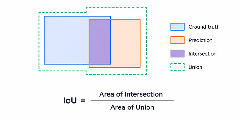
Detection metrics all begin with Intersection over Union. IoU is the overlap area between a predicted box and a ground truth box, divided by their combined area. A prediction counts as correct only if its IoU clears a threshold and its class is right.
| Metric | What It Measures | When to Look at It |
|---|---|---|
| IoU | Overlap between predicted and true box | Setting the correct threshold |
| Precision | Of everything detected, how much was real | When false alarms are costly |
| Recall | Of everything real, how much was found | When misses are costly, such as safety systems |
| AP | Area under the precision-recall curve for one class | Diagnosing per-class weakness |
| mAP@0.5 | Mean AP across classes at a loose IoU threshold of 0.5 | Did the model find the objects? |
| mAP@0.5:0.95 | Mean AP averaged over IoU thresholds from 0.5 to 0.95 | Are the boxes tight? This is COCO’s headline metric |
| AP_S / AP_M / AP_L | AP split by object area: under 32², 32² to 96², over 96² | Diagnosing small-object failure specifically |
The COCO protocol defines AP at IoU 0.50:0.05:0.95 as the primary challenge metric, with AP small, medium and large computed over those pixel area bands.
The most useful diagnostic is the gap between mAP@0.5 and mAP@0.5:0.95. A model at 0.89 mAP@0.5 and 0.52 mAP@0.5:0.95 is finding almost everything but placing boxes loosely. Sometimes that is the model. Often it is the training data, because the model learned box tightness from annotations that were not tight. Before retraining with a bigger backbone, pull 100 training images and measure box tightness by hand against the objects. It takes an afternoon and frequently explains the gap.
One caution on reported numbers. The benchmark itself is not perfect. A 2024 ECCV study inspected thousands of COCO masks and found imprecise boundaries, non-exhaustively annotated instances and mislabeled masks, then released COCO-ReM as a corrected annotation set. The authors evaluated fifty detectors against it. Models producing visually sharper predictions scored higher on the corrected labels, which means they had been penalized by errors in COCO-2017 rather than by their own mistakes.
A 2026 survey in Artificial Intelligence Review reaches a broader version of the same conclusion. Across MS COCO, Open Images, Pascal VOC, LVIS, Object365 and DOTA, it documents missing labels, misaligned boxes, inconsistent occlusion treatment and ambiguous category definitions as systematic rather than occasional problems.
If the field’s flagship benchmarks carry that much label noise, your in-house dataset almost certainly does too.
Why Detectors Fail in Production
A model at 0.92 mAP in validation can be useless in deployment. The failure patterns are consistent.
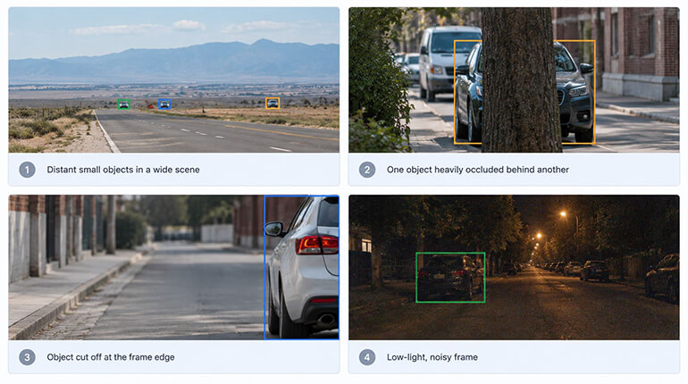
Small objects. After down-sampling, a 20-pixel object may occupy a single cell of the feature map. Higher input resolution, feature pyramid networks and tiled inference all help. So does a labeling policy that does not silently skip small objects.
Occlusion and crowding. Overlapping instances collide with NMS, as described earlier. Query-based detectors handle this better than anchor-based ones because they do not rely on suppression.
Class imbalance. If 94% of your boxes are one class, the model optimizes for that class and learns to ignore the rest. Rare-class recall will be poor no matter what the overall mAP says. Read per-class AP, not just the mean.
Domain shift. A model trained on daytime footage degrades at night, in rain, or on a different camera. This is a dataset composition problem. Training data needs to cover the conditions the system will actually meet, which is usually a data collection question before it is a labeling question.
Label noise. Missing labels are the most damaging kind, because an unlabeled object is not neutral. It is an explicit instruction that this appearance is background, and the model is penalized for detecting it correctly.
Temporal inconsistency in video. Frame-by-frame detection produces flickering identities across frames. If your product needs stable tracks, the annotation needs consistent object IDs across frames, which is a different and more demanding specification than per-frame boxes. Video annotation services handle this with interpolation between keyframes, and the tooling used has a large effect on both cost and ID consistency.
How Much Labeled Data You Need
There is no formula, but there are workable planning ranges for fine-tuning a pretrained detector.
| Scenario | Images per class | Notes |
|---|---|---|
| Proof of concept, visually distinct class | 300 – 500 | Enough to prove feasibility, not to deploy |
| Production, controlled environment | 1,000 – 3,000 | Fixed camera, stable lighting, limited variation |
| Production, variable real-world conditions | 2,000 – 10,000 | Multiple lighting conditions, angles, occlusion levels |
| Safety-critical or regulated | 10,000+ | Plus deliberate over-sampling of rare and dangerous cases |
Two adjustments matter more than the headline number. Variation beats volume: 2,000 images spanning every lighting condition, camera angle and occlusion level outperforms 10,000 near-duplicate frames from one shift. And rare cases need over-representation relative to their natural frequency, because a class appearing in 0.5% of frames will be learned poorly if you sample naturally.
The budget follows from box count, not image count. HabileData’s published data annotation cost benchmarks put bounding box work at an indicative $0.03 to $0.12 per box. A 5,000-image pilot averaging eight objects per image is 40,000 boxes, roughly $2,000 of labeling at $0.05 per box, and around $2,700 once guideline development, QA and project management are included. Those figures are indicative planning ranges rather than quotes, and density is the variable that moves them most. A crowded retail shelf image with 40 objects costs eight times what a three-object image costs, at identical per-box rates.
Run a paid pilot of 500 to 2,000 representative items, including your ugliest edge cases, before committing to a full dataset. Score it against a gold set your own team labels independently. A pilot is cheap. A 40,000-box dataset built on misunderstood guidelines is not.
Do Foundation Models Remove the Need for Labeling?
Partly, and not in the way the marketing suggests.
Open-vocabulary detectors accept free-text prompts instead of a fixed class list. Grounding DINO reports 52.5 AP on COCO without seeing any COCO images during training, and 63.0 AP on COCO test-dev after fine-tuning on COCO. YOLO-World-L reports 45.1 AP on COCO without COCO data. Those are genuinely impressive zero-shot numbers for general vocabulary.
They are also below what a fine-tuned detector achieves on a narrow domain, and the gap widens as your classes get further from everyday objects. A model that knows “car” and “person” from web-scale pretraining does not know your specific weld defect, your SKU packaging variant, or the difference between two visually similar surgical instruments.
Where these models earn their place is pre-labeling. The model drafts boxes, annotators correct them, and human time shifts from drawing to verifying. Pre-labeling with a reasonable model typically cuts human time by 30% to 70% on suitable tasks.
It carries a specific risk that is easy to miss. Annotators tend to accept the model’s suggestion, including its mistakes, because verifying is a lower-attention task than drawing. Systematic model errors then propagate into the ground truth and get reinforced in the next training round. The countermeasure is straightforward: seed gold-set items where the pre-label is deliberately wrong, and track how often annotators catch them. If catch rates fall, the review is becoming rubber-stamping.
Where Object Detection Is Used
| Industry | Application | Typical Detection Challenge |
|---|---|---|
| Automotive | Pedestrian, vehicle and sign detection | Occlusion, night conditions, safety-critical recall |
| Manufacturing | Defect detection, assembly verification | Small defects, extreme class imbalance |
| Retail | Shelf auditing, planogram compliance | Dense scenes, visually similar SKUs |
| Healthcare | Lesion and anomaly localization | Expert annotation required, low tolerance for misses |
| Agriculture | Crop, pest and yield monitoring | Cluttered backgrounds, variable lighting |
| Logistics | Package, pallet and container tracking | Motion blur, identity consistency across frames |
| Security | Intrusion detection, PPE compliance | False alarm cost, wide camera variation |
The pattern across these is consistent. The architecture choice is rarely the hard part. The hard part is a dataset that represents the deployment environment, labeled to rules that hold up under the messy cases.
Conclusion
Object detection is a well-solved problem at the architecture level. Pretrained models are open source, documented, and good enough that most teams can fine-tune something workable in a week.
What is not solved is the ground truth. Every coordinate a detector predicts is a reflection of coordinates a human drew, under rules someone wrote, checked by a process someone designed. When a detection model under-performs, the cause is more often in that chain than in the network.
So the sequence worth following is: define the classes a downstream decision actually needs, write the guidelines for occlusion, truncation and minimum size before labeling begins, pilot on a few hundred representative images, measure inter-annotator agreement, and only then scale. The architecture decision can wait. It is the easy one.
Frequently Asked Questions
Image classification assigns one label to a whole image. Object detection finds every instance of the target classes and returns a bounding box, class label and confidence score for each. Detection answers what and where; classification answers only what.
Through regression against human-drawn ground truth. During training the model compares its predicted coordinates with annotated boxes and adjusts weights to reduce the error. The annotated boxes are its only source of positional truth.
It depends entirely on the dataset. On COCO, the strongest real-time detectors currently sit around 55 to 60 mAP@0.5:0.95. On a narrow single-class industrial dataset, 0.90 mAP@0.5 is often reachable, and below 0.70 usually indicates a data problem rather than a model problem. Never compare mAP across different datasets.
For GPU deployment where accuracy leads, start with a query-based transformer detector such as RF-DETR. For CPU or edge deployment, start with a small YOLO variant. Then spend your remaining effort on the dataset, which will move your accuracy further than switching between modern architectures.
Around 300 to 500 annotated images per class for a proof of concept on a visually distinct class. Production systems in variable conditions typically need 2,000 to 10,000 per class. Coverage of conditions matters more than raw volume.
Down-sampling in the backbone leaves small objects with very little signal in the feature map. Annotation contributes as well, because annotators skip tiny or blurry objects more often than large ones, and every skipped object trains the model to treat that appearance as background. Check AP_S separately from overall mAP.
Use the one your training framework expects natively. COCO JSON for Detectron2 and MMDetection, YOLO txt for Ultralytics models, Pascal VOC XML for older pipelines. Conversion is routine, but verify the class index mapping on a sample after every conversion.
Indicatively $0.03 to $0.12 per box, so a 40,000-box dataset runs roughly $1,200 to $4,800 in labeling, plus 30% to 40% for guidelines, QA and project management. Object density per image drives the total far more than image count does.
Yes. A tight bounding box can be derived from a polygon or mask automatically. The reverse is not possible, which is why teams unsure about future requirements sometimes label polygons from the start and derive boxes as needed. That decision costs more up front and is worth weighing against the likelihood that you will actually need masks. The trade-offs between mask types are covered in this breakdown of semantic, instance and panoptic segmentation.
Planning a detection dataset and want the labeling spec right the first time?
Talk to our annotation team »

Biju Peter is a Senior Project Manager with 22+ years in the BPM industry, specializing in large-scale data operations and annotation-driven projects. He brings deep expertise in data processing, web research, scraping, and multi-modal annotation across image, text, audio, and video domains. He has successfully led 200+ projects, managed large teams, and delivered scalable, high-quality solutions for global AI and machine learning initiatives for clients across the globe. 🔗Connect with Biju on LinkedIn