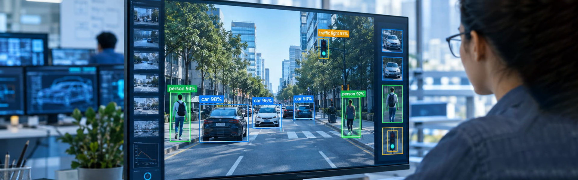

Computer vision is the field of AI that turns images and video into information software can act on. This guide covers the definition, the six-stage pipeline, the main task types and what each one outputs, real industry examples, realistic data volumes and annotation costs, and the reasons models that pass testing still fail in production.
Contents
- What Is Computer Vision?
- Key Takeaways
- Computer Vision vs Image Processing vs Machine Vision
- How Computer Vision Works, Stage by Stage
- The Core Computer Vision Tasks and What They Output
- The Training Data Layer Most Explainers Skip
- How Much Data Does a Computer Vision Model Need?
- Computer Vision Examples by Industry
- Why Computer Vision Models Fail in Production
- What Computer Vision Still Cannot Do Well
- How to Scope a Computer Vision Project
- The Short Version
- Computer Vision FAQs
What Is Computer Vision?
Computer vision is the field of artificial intelligence that enables software to extract usable information from images and video. A camera produces a grid of pixel values. A computer vision system converts that grid into something a program can act on: a class label, an object’s position, a measurement, a count, or a decision.
The phrase “teaching computers to see” gets used a lot. It is a fair metaphor and a poor description. Seeing is not the hard part. Cameras have been capturing pixels for decades. The hard part is interpretation, and interpretation is learned from examples rather than programmed.
That distinction matters because it determines where your project budget goes.
Key Takeaways
- Computer vision outputs information about image content. Image processing outputs another image. The two are often confused and frequently used together.
- Modern systems learn from labeled examples rather than hand-written rules, which is why the training data layer dominates project cost and timeline.
- The main task types are classification, object detection, segmentation, keypoint detection, and tracking. Each needs a different annotation type and is scored on a different metric.
- Published benchmark accuracy rarely survives contact with production data. Distribution shift is the usual culprit.
- Annotation is normally the largest single line item in a supervised vision project, ahead of compute.
Computer Vision vs Image Processing vs Machine Vision
These three terms get used interchangeably in vendor material, which causes real confusion during scoping. They are not the same thing.
| Computer vision | Image processing | Machine vision | |
|---|---|---|---|
| What it is | Scientific and engineering field concerned with interpreting visual data | Set of techniques for transforming image data | Industrial application of vision technology on a production line |
| Input | Image or video | Image | Image from a fixed, controlled camera setup |
| Output | Information: labels, coordinates, masks, measurements, decisions | Another image | A pass/fail signal, a measurement, or a robot instruction |
| Typical method | Trained neural networks, sometimes classical algorithms | Filters, transforms, histogram operations | Whichever of the two is more reliable and cheaper to maintain |
| Example | Identifying which products appear on a shelf photo | Removing noise from that photo before analysis | Checking bottle cap torque marks at 400 units per minute |
| Needs training data | Usually yes | No | Sometimes |
The practical version: if the answer comes out as a picture, that is image processing. If it comes out as information, that is computer vision. Machine vision is computer vision doing a factory job in controlled lighting, where the constraints are tight enough that classical methods often win.
One consequence is worth noting early. Not every vision problem needs a trained model. Barcode reading, fiducial alignment, and dimensional gauging on a jig are solved reliably by classical algorithms that need zero labeled data. Reach for deep learning when appearance varies in ways you cannot enumerate as rules.
How Computer Vision Works, Stage by Stage
Most explainers give you five stages: capture, preprocess, extract features, infer, act. That describes what happens when a finished model runs. It leaves out where the model came from, which is where the work is.
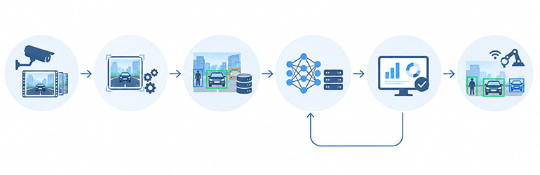
Here is the full picture.
Image acquisition. A sensor converts light into a digital array. For an RGB image, that is three values per pixel, each between 0 and 255. The choices made here set a ceiling on everything downstream. Resolution, frame rate, lens distortion, sensor noise, and lighting consistency all constrain what a model can learn. Teams routinely spend months tuning architectures to compensate for a camera that was mounted in the wrong place.
Preprocessing. Raw captures get normalized so the model sees consistent input: resizing, color space conversion, contrast adjustment, denoising, distortion correction. This is where classical image processing lives inside a modern vision pipeline. The same operations get applied at training time and at inference time, and a mismatch between the two is a common and annoying bug.
Annotation and dataset construction. Humans label what the model is supposed to learn. Boxes around objects, pixel masks around regions, points on joints, class names on whole images. This stage produces ground truth, and every accuracy number the project ever reports is measured against it. It is also, in most supervised projects, the longest and most expensive stage. More on it below.
Training. The model learns a mapping from pixels to labels by making predictions, measuring the error against ground truth, and adjusting its internal weights. In a convolutional network, early layers learn primitives such as edges and color gradients; deeper layers combine those into textures, parts, and eventually object-level patterns. Nobody tells the network what a wheel looks like. It infers wheel-ness from thousands of labeled examples.
Vision transformers, which now dominate many benchmarks, split the image into patches and use attention to weigh relationships between them instead of sliding filters across the grid. Different mechanism, same dependency on labeled data.
Evaluation. The trained model is scored on a held-out set it never saw during training. Classification uses accuracy, precision, recall, and F1. Detection uses mean average precision computed over Intersection over Union thresholds. Segmentation uses mean IoU or Dice coefficient. If you only ever see a single accuracy percentage quoted for a vision system, ask which metric and on which data, because the answer is often less flattering than the headline.
Inference and action. The deployed model receives new images and produces predictions, which some downstream system turns into behavior: flagging a defect, unlocking a phone, routing a package, braking a vehicle. Then the loop restarts, because production data drifts and models need retraining.
That evaluation-to-retraining loop is not a footnote. It is the difference between a demo and a system.
The Core Computer Vision Tasks and What They Output
“Computer vision” covers a family of tasks with very different costs and outputs. Choosing the wrong one is an expensive mistake, because the annotation you commission is task-specific and largely non-transferable.
| Task | Question it answers | Output | Annotation needed | Primary metric |
|---|---|---|---|---|
| Image classification | What is this a picture of? | One or more class labels per image | Image-level tags | Accuracy, F1 |
| Object detection | What objects are here and where? | Class plus bounding box coordinates | Bounding boxes | mAP at IoU thresholds |
| Semantic segmentation | Which pixels belong to which class? | Class label per pixel | Pixel masks | Mean IoU |
| Instance segmentation | Which pixels belong to which individual object? | Per-object pixel masks | Polygons or instance masks | Mask mAP |
| Keypoint detection | Where are the specific points on this object? | Ordered coordinate list | Landmark points | PCK, OKS |
| Object tracking | Where did this object go across frames? | Persistent IDs over time | Frame-level boxes with consistent IDs | MOTA, IDF1 |
| OCR and text recognition | What does this text say? | Transcribed strings with locations | Text regions plus transcription | Character and word error rate |
| Depth and 3D estimation | How far away is this? | Depth map or 3D coordinates | Stereo pairs, LiDAR point clouds, cuboids | RMSE, 3D IoU |
Detection and segmentation get conflated constantly. A bounding box tells you roughly where a car is. A segmentation mask tells you exactly which pixels are car. The first is cheap and adequate for counting and triggering. The second costs several times more per object and is necessary when boundaries carry meaning, as in tumor delineation or free-space mapping for a robot. Our breakdown of semantic vs instance vs panoptic segmentation covers where each variant earns its cost.
The Training Data Layer Most Explainers Skip
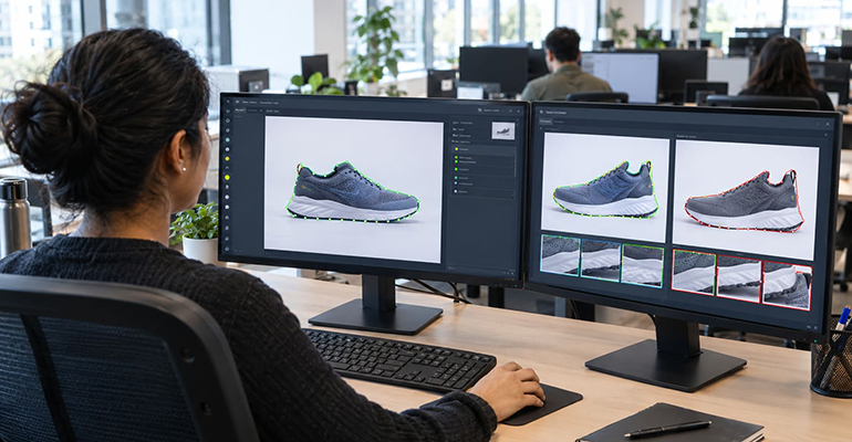
Here is the part that gets one sentence in most articles and eats most of the budget in most projects.
A supervised computer vision model knows exactly what its training labels taught it. Not more. If your dataset contains 40,000 images of retail shelves photographed in daylight, the model learns daylight shelves. If half the boxes are drawn 20% too large, the model learns to predict boxes 20% too large, consistently and confidently.
This is not a theoretical concern. A study of ten widely used ML benchmarks, including ImageNet, found an average of 3.3% label errors in their test sets, and correcting those errors changed which models ranked best. If the benchmarks the field measures itself against carry that much noise, an in-house dataset assembled under deadline pressure carries more.
Three things determine whether your ground truth is any good.
Guidelines. Written before labeling starts, not after the first batch comes back wrong. A guideline document that does not resolve occlusion, truncation at frame edges, minimum object size, and ambiguous class boundaries will produce inconsistent labels no matter how good the annotators are. Ambiguity in the spec is the single largest source of rework I see.
Review structure. A single annotation pass is the cheapest and least reliable option. A second review pass adds roughly 20 to 40% to labor cost. Consensus schemes, where several annotators label the same item independently and disagreements are adjudicated, can more than double it. Match the depth to what a wrong label costs you: full consensus on a product recommendation dataset is overkill, a single pass on pedestrian detection is reckless.
Measurement. Inter-annotator agreement tells you whether your guidelines are actually unambiguous. Spot-audit IoU against a gold-standard subset tells you whether the boundaries are tight enough. If you are not measuring either, you do not know your label quality, you are hoping. Our guide to image annotation quality metrics walks through how IoU, precision, recall, and F1 apply to annotation review specifically.
Scale makes this operational rather than academic. The COCO dataset, still a standard segmentation benchmark, contains 2.5 million labeled instances and consumed tens of thousands of annotator hours. Most commercial projects are smaller, but the same coordination problems appear at 50,000 images that appear at 2.5 million.
How Much Data Does a Computer Vision Model Need?
The honest answer is that it depends on class similarity, appearance variation, and how much failure costs you. The useful answer is a set of starting points.
With a pretrained backbone and transfer learning, which is how almost everyone starts:
- Classification, visually distinct classes: a few hundred to about 1,000 labeled images per class.
- Classification, visually similar classes: 2,000 to 5,000 per class. Distinguishing two similar defect types takes far more examples than distinguishing a cat from a truck.
- Object detection: roughly 1,500 to 5,000 labeled instances per class, not per image. A single street scene might contribute 30 instances.
- Semantic segmentation: fewer images often suffice, sometimes 500 to 2,000, because each image carries dense supervision. The annotation cost per image is five to twenty times higher.
- Keypoint detection: 5,000 to 10,000 annotated objects for reliable pose estimation, more if the object deforms.
Two adjustments matter more than the base numbers.
Rare classes need disproportionate representation. A defect occurring in 1 in 2,000 units will barely register in a randomly sampled dataset. You need targeted collection, oversampling, or both, or the model will learn that predicting “no defect” is 99.95% accurate and useless.
Variation beats volume. Ten thousand images from one camera under one lighting condition teach less than two thousand images spanning the cameras, times of day, and weather your system will actually encounter. When teams tell me their model tanked in production, the dataset was usually large and narrow.
Treat these as starting points for a pilot, not commitments. The reliable method is to label a slice, train, plot the learning curve, and see where accuracy starts to flatten. That tells you what the next batch is worth
Computer Vision Examples by Industry
Most articles list applications. Fewer explain what actually gets annotated to make them work, which is the part that determines feasibility.
Healthcare imaging. Detection and segmentation on X-ray, CT, MRI, and pathology slides. The FDA’s AI-Enabled Medical Device List recorded 1,451 authorized AI-enabled devices through the end of 2025, of which 1,104, about 76%, were reviewed by the radiology panel. Medical annotation is the expensive end of the market because it needs clinicians, region boundaries are genuinely ambiguous, and consensus review is mandatory rather than optional.
Autonomous vehicles and ADAS. Multi-sensor detection, segmentation, lane geometry, and 3D localization. Driving datasets are dense: hundreds of overlapping objects per frame, tight edge tolerances, and heavy occlusion. Annotation runs across camera images and LiDAR point clouds together, with cuboids in 3D matched to boxes in 2D.
Retail and ecommerce. Product recognition on shelves, planogram compliance, visual search, attribute tagging, and checkout-free store systems. The hard part is rarely the model. It is maintaining a taxonomy across tens of thousands of SKUs that change seasonally, with packaging refreshes that quietly invalidate your training set.
Manufacturing quality control. Defect detection and classification on production lines. Classic extreme class imbalance: thousands of good units per defect. Teams often do better with anomaly detection trained mostly on normal examples than with a conventional classifier starved of positive cases.
Agriculture. Crop and weed segmentation for precision spraying, yield estimation, disease identification from leaf imagery. Seasonal drift is brutal here. A model trained on one growth stage degrades on the next, so retraining cadence has to be planned into the operating budget.
Document and identity processing. OCR, layout parsing, signature and stamp detection, identity verification. Text detection plus transcription, with handwriting and multilingual content raising cost sharply.
Security and infrastructure. Intrusion detection, crowd density estimation, PPE compliance, traffic counting, structural inspection from drone imagery. Most of this runs on video, where frame-to-frame identity consistency matters more than per-frame precision. That is a video annotation problem with its own cost structure.
Consumer devices. Face unlock, portrait mode, scene detection, AR surface tracking, live translation. These run on-device, which means the model has to fit in a power and latency budget most server benchmarks ignore.
Why Computer Vision Models Fail in Production
A model that scores well on a held-out test set and then disappoints in deployment is the normal outcome, not an unlucky one.
Distribution shift is the leading cause. Production images differ from training images in ways nobody flagged: a new camera model, a repositioned mount, winter light instead of summer light, a repainted floor. The effect is measurable even under careful conditions. When researchers rebuilt the ImageNet test set following the original collection protocol as closely as they could, model accuracy dropped 11 to 14 percentage points across a wide range of architectures. That is the penalty for new images drawn from a deliberately similar distribution. Your production data is less similar than that.
Label noise caps accuracy invisibly. You cannot exceed the quality of your ground truth, and if the errors are systematic rather than random, the model learns the error as a rule.
Class imbalance produces models that are accurate and useless. Check per-class recall, never overall accuracy, when the classes are skewed.
Edge cases are absent by definition. The unusual pose, the partially occluded object, the reflective surface, the object at the frame boundary. These are rare in random samples and common in the failures that matter. Deliberate collection of hard cases beats more random data, every time.
Threshold and integration drift. The model may be fine while the confidence threshold, the tracking logic, or the downstream business rule quietly breaks. When accuracy “drops”, check the plumbing before retraining.
The countermeasure is unglamorous: monitor prediction distributions in production, sample and re-label a steady trickle of live data, and plan retraining as a standing cost rather than a surprise.
What Computer Vision Still Cannot Do Well
Worth saying plainly, because vendor material rarely does.
Causal and physical reasoning remains weak. A model can detect a ladder and a person on it without any notion that the ladder might fall. Fine-grained distinctions between visually near-identical categories still need far more data than intuition suggests. Performance under genuinely novel conditions is unreliable, and models tend to be confidently wrong rather than usefully uncertain. Adversarial and degraded inputs break systems that look robust on clean benchmarks. And explaining why a given prediction was made is still an open problem, which is a real constraint in regulated settings where “the model said so” is not an acceptable answer.
None of this makes computer vision less useful. It makes the difference between scoping a system that works and scoping one that demos well.
How to Scope a Computer Vision Project
- Write the decision first. Not “detect defects” but “flag units for manual inspection when surface scratches exceed 2mm”. The decision determines the task type, which determines the annotation, which determines the cost.
- Check whether you need learning at all. Fixed geometry and controlled lighting often yield to classical methods with no training data.
- Set the accuracy target against consequences. What does a false positive cost? A false negative? These numbers set your QA depth and your data volume, and they are usually very different from each other.
- Audit your data before collecting more. Most teams have more images than they think and less variety than they need.
- Run a labeled pilot. A few thousand images, properly annotated, trained and evaluated. This tells you whether the problem is tractable before you commission the full dataset.
- Lock the annotation guidelines. Include edge cases, positive and negative examples, and adjudication rules. Changing the spec mid-project means partial re-annotation.
- Scale annotation with QA proportional to risk. Single pass for low-stakes, multi-pass review for anything safety-relevant or regulated.
- Budget for retraining from day one. Drift is not a defect. It is the operating condition.
On costs, annotation usually dominates. At 2026 benchmarks, bounding boxes run about $0.03 to $0.12 per object and pixel-level segmentation about $0.20 to $1.50 per image, with onshore delivery typically two to four times higher. A 20,000-image detection dataset averaging six objects per image lands somewhere between $3,600 and $14,400 in labeling alone. Our image annotation pricing benchmarks break down where a quote’s money actually goes.
Pre-labeling is the highest-leverage saving. Run an existing model over your data to generate draft labels, then have annotators correct rather than draw from scratch. Correction is two to five times faster than cold labeling, and the saving compounds across every batch.
Frequently Asked Questions
It is software that turns pictures into information. A camera gives a computer a grid of numbers. Computer vision converts that grid into something actionable: a name, a location, a count, a measurement, or a decision.
No. Computer vision is one sub-field of artificial intelligence, specifically the one concerned with visual data. Natural language processing handles text, speech recognition handles audio. Many modern systems combine them, which is what “multi-modal” refers to.
No. Barcode reading, dimensional measurement on a jig, and fiducial alignment are handled reliably by classical algorithms with no training data at all. Deep learning earns its cost when appearance varies in ways you cannot write rules for.
It depends entirely on task, data, and conditions, and any single figure quoted without those is close to meaningless. Narrow tasks in controlled settings can exceed human consistency. The same model on uncontrolled real-world data can lose 10 or more percentage points. Always ask which metric, on which test set, collected when.
A pilot on a few thousand images is typically a few weeks including annotation. Production systems run three to nine months depending on dataset scale, regulatory requirements, and integration complexity. Annotation and iteration, not model training, usually set the timeline.
Machine vision is the industrial application: fixed cameras, controlled lighting, inspecting or guiding equipment. Computer vision is the broader field and includes uncontrolled environments where lighting, angle, and content vary freely.
Partially, and it should. Model-assisted pre-labeling is standard practice and saves substantial time. But automated labels degrade exactly where you need reliability most: rare classes, ambiguous boundaries, occlusion, and edge cases. Human review stays in the loop for anything consequential.
Data engineering to build and version datasets, ML engineering to train and evaluate models, domain expertise to define what a correct label means, and annotation operations to produce ground truth at volume with measurable quality. Most teams underestimate the last one and end up rebuilding it mid-project.
Working on a computer vision project and need the training data behind it?
Talk to an annotation specialist »

Biju Peter is a Senior Project Manager with 22+ years in the BPM industry, specializing in large-scale data operations and annotation-driven projects. He brings deep expertise in data processing, web research, scraping, and multi-modal annotation across image, text, audio, and video domains. He has successfully led 200+ projects, managed large teams, and delivered scalable, high-quality solutions for global AI and machine learning initiatives for clients across the globe. 🔗Connect with Biju on LinkedIn