A practical guide to YOLO object detection: how the single-pass architecture works, what changed across versions from YOLOv1 to YOLO26, what published latency numbers mean on real hardware, and how to prepare, convert and QA the label files YOLO training actually requires.
Contents
- Key Takeaways
- What Is YOLO Object Detection?
- How YOLO Works In A Single Pass
- YOLO Versions: What Actually Changed
- YOLO Speed Benchmarks And What They Mean
- Will It Hit Your Frame Rate?
- The YOLO Label Format Explained
- Dataset Structure And data.yaml
- Converting COCO And Pascal VOC To YOLO
- Annotation Rules That Decide Detection Accuracy
- Label Defects And How To Catch Them
- How Much Training Data Do You Need?
- Choosing A YOLO Version
- When YOLO Is The Wrong Tool
- Conclusion
- Frequently Asked Questions
YOLO is the default answer when someone needs object detection to run in real time. It is also one of the most misunderstood choices in computer vision, because the part that decides whether it works is not the architecture. It is the label file.
This guide covers all three things a team needs before committing: what YOLO does, what actually changed across versions, and what the training data has to look like.
Key Takeaways
- YOLO predicts every bounding box and class in one forward pass, which is why it is fast enough for video.
- The version list is long and no longer sequential. YOLO26, released January 2026, is the current Ultralytics release.
- Published latency figures measure model inference only. Decoding, resizing and drawing are yours to budget for.
- YOLO labels are one text file per image, one line per object, with all coordinates normalized to 0-1.
- Most failed YOLO projects fail on the labels, not the model. Conversion errors and inconsistent annotation rules are silent.
What Is YOLO Object Detection?
YOLO (You Only Look Once) is a family of single-stage object detection models that predict all bounding boxes and class labels for an image in one forward pass of a neural network. Earlier detectors such as R-CNN proposed candidate regions first and classified each one separately. YOLO removed that second stage, which is what made real-time detection on video practical.
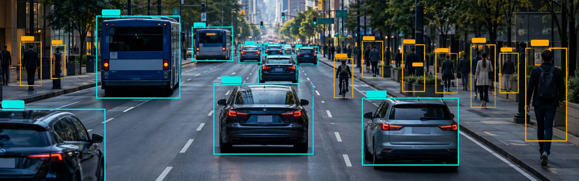
The output for each detected object is a rectangle, a class label and a confidence score. That is all. YOLO does not tell you an object’s exact outline, only the box that contains it.
The original model, published by Joseph Redmon and colleagues in 2015, ran at 45 frames per second while reaching 63.4 mAP on Pascal VOC. That combination was the point. Detection accuracy at the time was achievable; detection accuracy at video frame rates was not.
How YOLO Works In A Single Pass
The mechanics have changed substantially across versions, but the shape of the process has not.
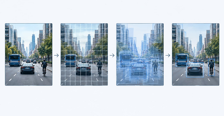
- The image is resized to a fixed input size, usually 640 by 640 pixels, with padding to preserve aspect ratio.
- A convolutional backbone extracts features at several scales, so that both a truck and a distant traffic sign have a feature map suited to their size.
- A detection head predicts densely. Every spatial position across those feature maps emits candidate box coordinates, an objectness score and class scores. The image is effectively divided into a grid, and each cell is responsible for the objects centered in it.
- Overlapping candidates are reduced to final detection. Historically this was Non-Maximum Suppression, a post-processing step that keeps the highest-scoring box and discards others that overlap it beyond an IoU threshold.
- A confidence threshold filters the rest.
Step 4 is where recent versions diverge. NMS is a sequential operation whose cost depends on how many objects are in the frame, which makes latency unpredictable and complicates export to edge accelerators. YOLOv10 first demonstrated a YOLO model that removes it by training the network to emit one prediction per object directly. YOLO26 makes that end-to-end behavior the default across detection, segmentation, pose and oriented box tasks.
One consequence matters operationally: an NMS-free model has constant-time post-processing regardless of object count. A crowded frame no longer costs more than an empty one.
YOLO Versions: What Actually Changed
The version list is not a clean sequence. Different groups have released models under the YOLO name, numbering has jumped, and the newest Ultralytics release switched to a year-based name.
| Version | Year | Released by | The change that mattered |
|---|---|---|---|
| YOLOv1 | 2015 | Redmon et al., University of Washington | Single-pass detection as one regression problem |
| YOLOv2 / YOLO9000 | 2016 | Redmon & Farhadi | Anchor boxes and batch normalization for stable box prediction |
| YOLOv3 | 2018 | Redmon & Farhadi | Darknet-53 backbone and multi-scale prediction |
| YOLOv4 | 2020 | Bochkovskiy et al. | CSPDarknet53, mosaic augmentation, a wide bag of training tricks |
| YOLOv5 | 2020 | Ultralytics | PyTorch implementation and a usable training CLI |
| YOLOX | 2021 | Megvii | Anchor-free detection head |
| YOLOv6 | 2022 | Meituan | Re-parameterized backbone aimed at industrial deployment |
| YOLOv7 | 2022 | Wang et al. | Trainable bag-of-freebies and model scaling |
| YOLOv8 | 2023 | Ultralytics | Anchor-free C2f architecture, decoupled head, unified multi-task API |
| YOLOv9 | 2024 | Wang et al. | Programmable gradient information and GELAN |
| YOLOv10 | 2024 | Tsinghua University | First YOLO to remove NMS, via dual label assignment |
| YOLO11 | 2024 | Ultralytics | Refined accuracy and efficiency across all five model scales |
| YOLOv12 | 2025 | Tian et al. | Attention-centric design with R-ELAN blocks |
| YOLO26 | 2026 | Ultralytics | Native NMS-free inference, DFL removal, MuSGD optimizer, small-object loss |
YOLO26 arrived on 14 January 2026 and reports 40.9 to 57.5 mAP on COCO across its five scales at 1.7 to 11.8 ms latency on a T4 GPU with TensorRT. Ultralytics has since opened a wait-list for YOLO27, so this table will need revisiting.
Two things are worth pulling out for anyone planning a project.
Numbering does not imply lineage. YOLOv9 and YOLOv12 came from academic groups, YOLOv10 from Tsinghua, and the v5, v8, 11 and 26 line from Ultralytics. A higher number does not guarantee the tooling, export paths or documentation your team is used to.
Licensing differs by version. Ultralytics publishes its code under AGPL-3.0 alongside a paid commercial license. AGPL carries source disclosure obligations that apply to software delivered over a network, which is exactly how most detection systems are shipped. Other YOLO variants use different terms. This is a legal question, not an engineering one, and it belongs in the evaluation before training starts rather than after.
YOLO Speed Benchmarks And What They Mean
Published figures for the current Ultralytics models, measured at 640 pixel input on COCO:
| Model | mAP 50-95 | CPU ONNX (ms) | T4 TensorRT (ms) | Params (M) |
|---|---|---|---|---|
| YOLO26n | 40.9 | 38.9 | 1.7 | 2.4 |
| YOLO26s | 48.6 | 87.2 | 2.5 | 9.5 |
| YOLO26m | 53.1 | 220.0 | 4.7 | 20.4 |
| YOLO26l | 55.0 | 286.2 | 6.2 | 24.8 |
| YOLO26x | 57.5 | 525.8 | 11.8 | 55.7 |
| YOLO11n | 39.5 | 56.1 | 1.5 | 2.6 |
| YOLO11m | 51.5 | 183.2 | 4.7 | 20.1 |
| YOLOv8n | 37.3 | 80.4 | 1.47 | 3.2 |
| YOLOv8m | 50.2 | 234.7 | 5.86 | 25.9 |
Read these carefully, because they are easy to over-claim from.
The CPU numbers come from one specific processor. Ultralytics measured on an Intel Xeon at 2.00 GHz using ONNX. A Raspberry Pi, an ARM laptop and a modern desktop CPU will all produce different results, and the ranking between models can shift.
The headline speedup and the table do not match exactly. Ultralytics states up to 43% faster CPU inference for YOLO26n against YOLO11n. The per-model table shows 38.9 ms against 56.1 ms, which is roughly 31%. Against YOLOv8n at 80.4 ms it is closer to 52%. “Up to” is doing work in that sentence. Benchmark your own export on your own hardware before committing to a latency SLA.
NMS-free costs a little accuracy. Ultralytics reports the one-to-one head giving up 0.6 to 0.8 mAP on COCO compared with the traditional head, in exchange for dropping the NMS pass. You can switch back if accuracy matters more than deterministic latency.
These are inference times only. They exclude video decoding, resizing and letterboxing, tensor transfer, drawing and any tracking logic. In production pipelines those stages routinely consume as much time as the model.
Will It Hit Your Frame Rate?
Convert latency to a frame budget rather than trusting an FPS headline.
A 30 FPS camera gives you 33.3 ms per frame for everything.
- YOLO26n on the benchmarked CPU: 38.9 ms of inference alone. Already over budget before decoding a single frame.
- YOLO11n on the same CPU: 56.1 ms. Roughly 18 FPS at best.
- YOLO26n on a T4 with TensorRT: 1.7 ms, leaving 31 ms for everything else. Comfortable.
Three practical adjustments when the budget is tight:
- Drop the input size. Moving from 640 to 416 pixels cuts compute substantially. It also hurts small-object recall, which may or may not matter for your classes.
- Do not run detection on every frame. Detect every third or fifth frame and track between them. For most surveillance and retail analytics work this is invisible in the output.
- Export properly. The gap between raw PyTorch and a tuned TensorRT or OpenVINO export is often larger than the gap between two model versions.
The YOLO Label Format Explained
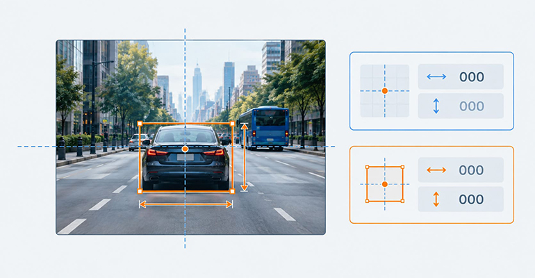
The YOLO annotation format is one plain text file per image, sharing the image’s filename, with one line per object in the form class_id x_center y_center width height. All four coordinates are normalized to the range 0 to 1 by dividing by the image width and height. Class IDs are zero-indexed. An image containing no objects needs no label file.
That is the whole specification. The failure modes come from what it leaves implicit.
A Worked Example
Take a 1920 by 1080 image with one car. In pixels, the box runs from (800, 300) at top left to (1100, 700) at bottom right.
Box width: 1100 − 800 = 300 px Box height: 700 − 300 = 400 px Centre X: 800 + 300/2 = 950 px Centre Y: 300 + 400/2 = 500 px
Normalize against the image dimensions:
x_center = 950 / 1920 = 0.494792 y_center = 500 / 1080 = 0.462963 width = 300 / 1920 = 0.156250 height = 400 / 1080 = 0.370370
If car is class 2, the line in image_0001.txt is:
2 0.494792 0.462963 0.156250 0.370370
The same object in the two formats you are most likely converting from:
| Format | How this box is stored | Units | Class handling |
|---|---|---|---|
| YOLO TXT | 0 0.194792 0.462963 0.156250 0.370370 |
Normalized 0-1, centre-based | Zero-indexed integer, order fixed by data.yaml |
| COCO JSON | "bbox": [800, 300, 300, 400] |
Pixels, top-left corner plus width and height | category_id, can start at any number and skip values |
| Pascal VOC XML | <xmin>800</xmin><ymin>300</ymin><xmax>1100</xmax><ymax>700</ymax> |
Pixels, two corners | Class name as a string |
Three different conventions for one rectangle. Every one of the common conversion bugs lives in this table: corner versus centre, pixels versus normalized, and string class names versus integer indices.
Dataset Structure And data.yaml
YOLO training expects images and labels in parallel directories, matched by filename:
my_dataset/
├── images/
│   ├── train/
│   │   └── image_0001.jpg
│   └── val/
├── labels/
│   ├── train/
│   │   └── image_0001.txt
│   └── val/
└── data.yaml
The configuration file declares the dataset root, the split paths and the class list:
yaml

path: my_dataset
train: images/train
val: images/val
test:
names:
  0: person
  1: bicycle
  2: car
The order of names is the contract. Index 2 means car because it is third in this list, not because anything in the label files says so. Reorder the list after labeling and every annotation in the dataset silently changes meaning. Version this file with the same discipline you apply to code.
Converting COCO And Pascal VOC To YOLO
Ultralytics ships a converter for COCO-format annotations:
python

from ultralytics.data.converter import convert_coco
convert_coco(
    labels_dir="my_dataset/annotations/",
    save_dir="my_dataset/converted/",
    cls91to80=False,
)
The procedure, whether you use that function or write your own:
- Map category IDs to a contiguous zero-indexed list. COCO category IDs are not required to start at 1 or run without gaps. The
cls91to80flag exists because the original COCO release used 91 category IDs for 80 classes. Leaving it enabled on a custom dataset remaps your classes to COCO’s, which is the single most common reason a converted dataset trains to near-zero mAP. - Convert each box from
[x_min, y_min, width, height]in pixels to normalized centre form using the arithmetic above. - Write one text file per image, named to match the image exactly, including case.
- Skip crowd and zero-area annotations. COCO’s
iscrowd: 1regions describe groups rather than single instances and will teach the model the wrong thing if treated as normal boxes. - Write data.yaml with the class names in the exact index order used in step 1.
- Verify before training. Render the converted labels back onto a random sample of images and look at them. Twenty images will catch almost every systematic conversion error, and this step takes ten minutes.
Pascal VOC XML needs the same treatment plus a name-to-index mapping, since VOC stores class names as strings. Ultralytics tooling detects VOC labels but does not import them directly, so plan for a conversion step.
Annotation Rules That Decide Detection Accuracy
Format conversion is mechanical. The decisions that separate a dataset that trains well from one that does not are made by annotators, one object at a time, and they only stay consistent if the guidelines say what to do.
After running annotation programmes across image, video and LiDAR datasets, the same handful of ambiguities surface on nearly every detection project. Each one needs an explicit rule before labeling starts.
Truncation at the image border. Does a car half outside the frame get a box covering only its visible part, or the estimated full extent? Both are defensible. Mixing them within a dataset teaches the model that box edges are arbitrary. State one rule.
Occlusion. When a pedestrian is 70% hidden behind a vehicle, is that one box around the visible region, one box around the inferred whole person, or no box at all? Set a visibility threshold in percentage terms, below which the object is skipped, and hold everyone to it.
Tightness. A box drawn with several pixels of margin around every object systematically shifts what the model learns a boundary looks like. Our image annotation work is benchmarked against a 95%+ IoU threshold for bounding boxes precisely because this error is invisible in review and compounds across every training iteration.
Crowds and groups. Twenty people at a distance: individual boxes, one group box, or an ignore region? Individual boxes on tiny distant objects are expensive and often inconsistent. Decide based on whether your application actually needs to count them.
Class taxonomy. Is a pickup a car or a truck? Is a parked bicycle still a bicycle? Ambiguous class boundaries produce disagreement between annotators that no amount of QA can clean up afterwards, because there is no correct answer to check against.
Background images. Images containing none of your classes are useful training data. They teach the model what not to fire on. YOLO accepts them as images with no corresponding label file, and a modest proportion of them reduces false positives in deployment.
The practical test for any guideline: hand it to two annotators who have not discussed it, give them the same fifty images, and measure their agreement. Where they diverge, the guideline is ambiguous, not the annotators. That measurement is worth running before the main batch starts rather than after.
Detailed technique selection, including where bounding boxes stop being sufficient, is covered in our image annotation guide.
Label Defects And How To Catch Them
Training does not fail loudly on bad labels. It produces a number that looks plausible and a model that does not work. This table maps what you see to what usually causes it.
| Symptom | Likely cause | How to confirm |
|---|---|---|
| mAP near zero from the first epoch | Coordinates left in pixels, not normalized | Check whether any value in a label file exceeds 1.0 |
| Boxes consistently offset in one direction | Converter used corner coordinates as centre | Render labels onto images and look |
| One class never predicted | Class index mismatch between labels and data.yaml | Count instances per class ID against the names list |
| All classes predicted as the wrong class | Off-by-one in category remapping | Render five images per class and check the labels |
| Training runs but sees no objects | Image and label filenames do not match | Compare file stems in images/ and labels/ directories |
| High training mAP, poor validation mAP | Near-duplicate frames split across train and val | Check whether consecutive video frames appear in both |
| Good mAP overall, one class unusable | Severe class imbalance | Count instances, not images, per class |
| Erratic accuracy on the same class | Ambiguous guideline resolved differently by different annotators | Sample and measure inter-annotator agreement |
The last row is the one teams underestimate. It does not appear in any automated validation because every individual label is well-formed. It only shows up as a model that is inexplicably weaker on one class, and it is only fixable by rewriting the guideline and relabeling.
Automated checks catch the top of this table cheaply: value ranges, filename matching, class ID bounds, per-class instance counts, and boxes with zero or negative area. Run them as a gate before training, not as a diagnosis afterwards.
Teams frequently underestimate the QA layer when planning annotation effort. Boxes are quick to draw, averaging a few seconds per object, and it is easy to size a project on drawing time alone. Review, correction and agreement measurement are where the schedule actually goes, and our bounding box annotation services are structured around that reality rather than raw throughput.
How Much Training Data Do You Need?
There is no universal figure, and anyone who gives you one without asking about your classes is guessing.
What actually drives the requirement:
- Instances per class, not images. A thousand images containing one object each is a thousand instances. The same thousand images of crowded scenes might hold fifty thousand. Count instances.
- Visual variability. A fixed camera watching a conveyor belt under constant lighting needs far less data than a dashcam across seasons, weather and times of day.
- Class similarity. Separating sedan from hatchback needs far more examples than separating car from person.
- Object size. Small objects are harder. Datasets dominated by distant, few-pixel targets need more of them, and benefit from versions with small-object-specific training such as YOLO26.
- Class balance. A rare class with a hundred instances against a common class with fifty thousand will be under-served no matter how large the dataset is overall.
A workable approach: fine-tune a pretrained model on a small pilot set, plot validation mAP, then double the data and measure again. If the curve is still climbing steeply, keep labeling. If it has flattened, more of the same data will not help and the problem is elsewhere, usually in label consistency or class definitions.
Pre-labeling with an existing model and correcting the output is worth doing once you have a model that is roughly competent. It reduces effort substantially on repetitive classes. It also introduces a specific risk: reviewers correct what is obviously wrong and accept what looks approximately right, so boxes drift towards slightly loose. Measure IoU against a gold-standard set periodically rather than assuming review caught it.
Choosing A YOLO Version
| Your situation | Reasonable choice |
|---|---|
| New project, CPU or edge hardware | YOLO26, built for that case |
| New project, GPU available, want maturity | YOLO11, widely deployed and well-documented |
| Existing production pipeline on YOLOv8 | Stay unless you have a measured reason to move |
| Strict deterministic latency requirement | An NMS-free model, YOLO26 or YOLOv10 |
| Many small objects, aerial or drone imagery | YOLO26, whose loss design targets small targets |
| AGPL is a blocker | A commercial license, or a differently licensed variant |
| Publishing research | Whatever your reviewers accept as a baseline |
When YOLO Is The Wrong Tool
YOLO outputs rectangles. If your application needs something else, no version of it will help.
- Pixel-exact boundaries. Measuring area, cutting out objects or analyzing shape needs segmentation masks, which means polygon annotation rather than boxes.
- Rotated objects. Ships in satellite imagery, text on packaging and objects on a conveyor at arbitrary angles fit a rectangle poorly. Oriented bounding box variants exist for this.
- Very small objects in very large images. Detecting a hairline crack in a 10,000 pixel inspection scan usually needs a tiling strategy, not a bigger model.
- Detecting classes you never labeled. Closed-vocabulary detectors only find what was in the training set. Open-vocabulary models handle the case where new classes arrive constantly.
Choosing the annotation type is really choosing the model output you need, which is why that decision belongs at the start of a project. Our image annotation services cover bounding box, polygon, segmentation, keypoint and 3D cuboid labeling, delivered in COCO JSON, Pascal VOC XML, YOLO TXT and PNG mask formats, so the format follows the architecture rather than constraining it.
Conclusion
YOLO is a good default for real-time detection, and the current generation removed the post-processing step that used to make latency unpredictable. Picking the version is the straightforward part: benchmark two scales on your own hardware with your own export format and take the smaller one that clears your frame budget.
The part that decides whether the project works is the dataset. The format itself is simple enough to describe in one sentence. Getting a hundred thousand objects labeled to a consistent standard, with boundary rules that hold across a team and a QA layer that measures agreement rather than assuming it, is the actual engineering problem. That is the work worth planning carefully.
Frequently Asked Questions
You Only Look Once. The image passes through the network a single time and every bounding box and class is predicted at once, rather than proposing candidate regions first and classifying them in a second stage.
For new projects on CPU or edge hardware, YOLO26 is the current Ultralytics release and is designed for that case. YOLO11 remains a strong, widely deployed choice with more community material behind it. Stay on an older version only when an existing pipeline is tightly coupled to its outputs or license terms.
One plain text file per image, named to match the image. Each line is class_id x_center y_center width height, with all four coordinates normalized to 0-1 by dividing by image width and height, and class IDs zero-indexed. Images with no objects need no file.
Remap category IDs to a contiguous zero-indexed list, convert each box from pixel corner-plus-size to normalized centre form, write one text file per image, and create a data.yaml with the class names in that same order. Ultralytics provides convert_coco(), and its class-mapping flag must be set to False for custom datasets or your classes will be remapped to COCO’s.
There is no fixed number. Fine-tuning a pretrained model on a narrow, visually consistent task can work with a few hundred instances per class. Broad classes, cluttered scenes, variable lighting and small objects push that into the thousands. Count instances per class rather than images, and grow the dataset until the validation curve flattens.
It depends on the version. Ultralytics releases its code under AGPL-3.0, which carries source disclosure obligations for software delivered over a network, alongside a paid commercial license. Other YOLO variants use different licenses. Confirm the terms of the specific repository and weights with your legal team before deployment.
Usually a silent data defect rather than a hyper-parameter. Check for coordinates left in pixels, class IDs offset by one during conversion, image and label filenames that do not match, near-duplicate frames split across train and validation, and classes with too few instances to learn. Rendering labels back onto a sample of images catches most of these in minutes.
Yes, and they help. Images containing none of your classes teach the model what not to fire on and reduce false positives in deployment. YOLO handles them as images with no corresponding label file.
Need annotated training data for a detection model?
Get a free pilot »

Biju Peter is a Senior Project Manager with 22+ years in the BPM industry, specializing in large-scale data operations and annotation-driven projects. He brings deep expertise in data processing, web research, scraping, and multi-modal annotation across image, text, audio, and video domains. He has successfully led 200+ projects, managed large teams, and delivered scalable, high-quality solutions for global AI and machine learning initiatives for clients across the globe. 🔗Connect with Biju on LinkedIn